Two - Dimensional Lid - Driven Cavity Flow - Creeping Flow

Example 13.1 - Two - Dimensional Lid - Driven Cavity Flow - Creeping Flow

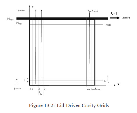
Consider a two dimensional square cavity filled with an incompressible fluid as shown in Figure 13.1. A steady creeping fluid motion is generated inside the cavity by the slid of the infinitely long top lid at a constant velocity U0. Since there is no fluid squeezed out of the cavity below the moving plate, the momentum, or vorticity, generated at the upper wall is diffused into the fluid forming closed path patterns within the cavity. We want to find this pattern.

From the hydrodynamics point of view, this problem represents a simplified model of complicated flow phenomena like recirculating flows in the lubrication process or flow in micro - structures.

Working with nondimensional equations, we may assume the size of the cavity is 1 × 1 and the sliding velocity is U₀ = 1

Simplified Staggered Grid

The regular approach of single grid will create some difficulties in these problems. Here, vorticity and velocities are given in terms of the derivatives of stream function. With a regular grid for vorticity, stream function and velocities on the faces of the control volumes should be approximated. Such an approximation will increase the errors.

A convenient way to get around these complications is to use two different grids. The first grid is our regular grid. We use this grid for the vorticity. The second grid is staggered towards left to coincide with the boundaries of the control volumes. This grid is used for the stream function. This is a simple model of the staggered grids which will be used later in solving convective - diffusive flows.

On this basis, we find the vorticity by solving a conservation of momentum. Then, the stream function can be found by solving the Poisson Equation, using a finite difference method. Notice that the values of the stream function are set on the second grid. Finally, having the stream function, we can find the velocities from Eqn.(13.2).

To distinguish between the two grids, the grid for vorticity is indexed by i and j and the second grid by I and J. The west walls of the cavity will be defined by I = 1 and J = 1. Assuming a uniform grid with Δ x = Δ y = h, the grids can be presented as in Figure 13.2.

The Integral Equations

The governing equations are shown in Eqns.(13.1) and (13.2). The vorticity equation (Eqn.(13.1)) is exactly like the heat conduction equation. This is an elliptic differential equation and the value of the vorticity should be preassigned on all boundaries. Hence, the integral equation given in the Eqn.(7.25) can be used here.

Boundary conditions

Assigning the vorticity on the walls is not always straight forward. Here we find the vorticity on the walls by the use of Eqn.(13.3) as follows

The north wall
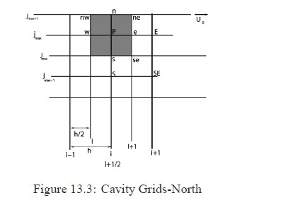
A schematic drawing of a typical north boundary grids is shown in Figure 13.3.

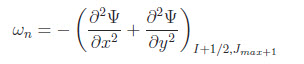
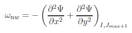
The vorticity on the north wall is given by

It is clear, from Figure 13.3, that the north control volumes are indexed by (i, j_max+1) and the north wall by (I + 1/2, J_{max + 1}). Then we can write

On the wall, we can assume

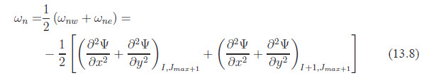
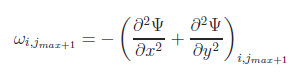
First, let us consider the vorticity at (I, J_{max + 1}), we have

It is not difficult to show that if we use the Taylor’s series expansion for the right - hand side terms, we can get a proper difference equation:

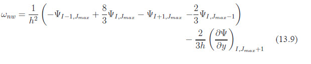
Knowing

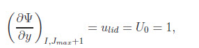
Eqn.(13.9) can be written as

Similarly we can write:

Then, Eqn.(13.8) can be written as
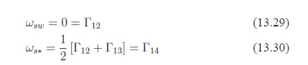
The west wall
We have (see the book for the derivation)
The east wall: See the book
The south wall: See the book

Discretization

Vorticity Equation (for detail of derivation see the Book)
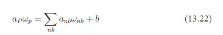
Here we formulate our discretization (similar to Example 8.6), in the form of
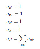
1. The Inner Nodes, defined by: {2 ≤ i ≤ i_max − 1, 2 ≤ j ≤ j_max − 1}
  and, from Eqn.(13.7), we have
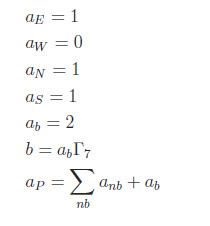
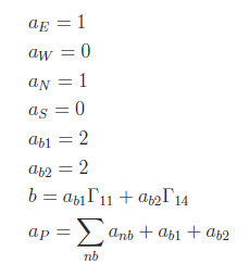
2. The West Boundary, defined by: {i = 1, 2 ≤ j ≤ j_max−1}
  Here, we have a Dirichlet boundary condition. Then (see the book for the derivation)
3. The North Boundary, defined by {j = j_max, 2 ≤ i ≤ i_{max_−1}} Then (see the book)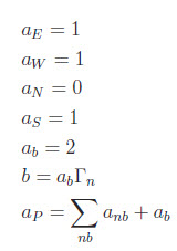
4. The East Boundary: See the Book
5. The South Boundary: See the Book
6. SW Corner defined by: {i = 1, j = 1}
  The schematic of the southwest cell is shown in Figure 13.7.
  
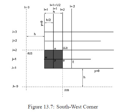
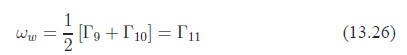
  On the west side we have:
  
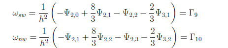
  Here we have a ghost cell at (2, 0). The easiest way to approximate the value of at this point is to use a linear extrapolation based on Ψ_2,1 and Ψ_2,2. But we know that Ψ_2,1 is on the wall, hence it is zero. Then we have
  Ψ_2,0 = - Ψ_2,2
  That is
  Γ₉ = 0
  Hence
  
  For the south side we have
  
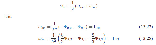
  The ghost point here is at (0, 2). Using the same argument we can say
  Ψ_2,0 = - Ψ_2,2
  Hence
  
  Then (see the Book)
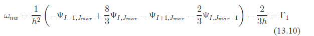
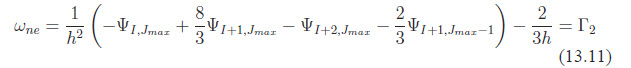
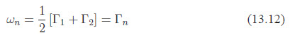
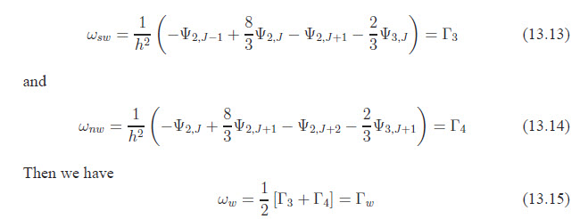
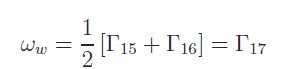
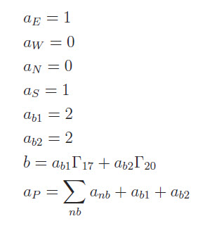
7. NW Corner, defined by {i = 1, j = j_max}
  Here, we have
  
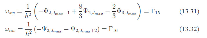
  and
  
  Similarly
  
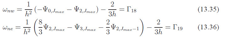
  and
  
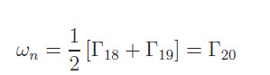
  Finally
Stream-Function
For the stream - function we have:
∇² = - ω
The value of the stream - function on all the boundaries are equal to zero. Hence, this equation should be solved for the interior points of the (I, J) grid.
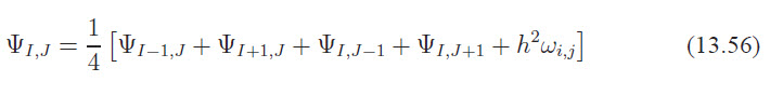
The stream - function Ψ is not a conserved variable. Hence, we can use a 2nd - order finite difference approximation for Eqn.(13.55). Then, we will have:

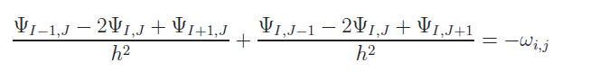
Then the finite difference discretization would be
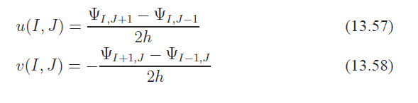
Velocities
We have

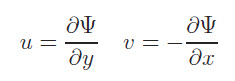
Then, using a 2nd - order approximation, we will have